Completing SentinelMesh: LSTM Anomaly Detection and Security Dashboarding
In Part 2, I trained a 1D-CNN to classify IoT network flows as benign or malicious.
That model worked well as a binary attack classifier, but it had one limitation: it was reactive. It looked at a flow and decided whether that flow looked malicious.
For SentinelMesh, I also wanted a proactive signal.
That is where the LSTM comes in.
The LSTM asks a different question:
Is the current traffic rate behaving abnormally compared to normal IoT behavior?
Why add an LSTM?
Some attacks do not start as a single obvious malicious flow. Flood attacks, scanning, and botnet behavior can first appear as abnormal changes in volume or rate.
A CNN can classify individual flows. An LSTM can watch behavior over time.
Together:
CNN  = What does this flow look like?
LSTM = Is the traffic pattern behaving normally?
That combination gives SentinelMesh both reactive and proactive detection.

Step 1: Train only on benign traffic
The LSTM was trained only on benign traffic.
Why?
Because the goal was to teach the model what normal looks like. Then, during live traffic, large prediction errors can become anomaly signals.
df_benign = df[df["is_attack"] == 0].reset_index(drop=True)
rate_series = df_benign["Rate"].values.reshape(-1, 1)
For this model, I focused on the Rate feature, which represents traffic rate in packets per second.
Step 2: Scale the rate values
from sklearn.preprocessing import MinMaxScaler

rate_scaler = MinMaxScaler(feature_range=(0, 1))
rate_scaled = rate_scaler.fit_transform(rate_series).astype("float32")
This was useful, but it also introduced one of the biggest lessons from the project: time-series models are extremely sensitive to scaling and outliers.
More on that in a minute.
Step 3: Create sequences
The LSTM used a sliding window of 30 previous rate values to predict a future rate value.
Input:  previous 30 rate values
Output: predicted future rate value
Prediction horizon: 5 steps ahead
seq_length = 30
prediction_horizon = 5

seq_arrays = []
seq_labs = []

for i in range(len(rate_scaled) - seq_length - prediction_horizon):
    input_seq = rate_scaled[i : i + seq_length]
    label = rate_scaled[i + seq_length + prediction_horizon - 1]
    seq_arrays.append(input_seq)
    seq_labs.append(label)
Step 4: Preserve time order
For normal classification problems, shuffling is usually fine. For time series, order matters.
So instead of randomly splitting the data, I split the sequences chronologically.
split_idx = int(len(seq_arrays) * 0.8)

train_X = seq_arrays[:split_idx]
train_y = seq_labs[:split_idx]

val_X = seq_arrays[split_idx:]
val_y = seq_labs[split_idx:]
Step 5: Build the LSTM model
from tensorflow.keras import layers, models
import tensorflow as tf

model_lstm = models.Sequential([
    layers.LSTM(64, input_shape=(30, 1), return_sequences=True),
    layers.Dropout(0.2),

    layers.LSTM(32, return_sequences=False),
    layers.Dropout(0.2),

    layers.Dense(1),
    layers.Activation("linear")
])

model_lstm.compile(
    loss="mean_squared_error",
    optimizer=tf.keras.optimizers.Adam(learning_rate=0.001),
    metrics=["mse"]
)
This model predicts a continuous value, not a class label.
So instead of asking whether traffic is benign or malicious, it predicts the expected traffic rate.
Step 6: Evaluate the LSTM
The LSTM converged to a low normalized MSE, but the raw-scale results revealed a problem.
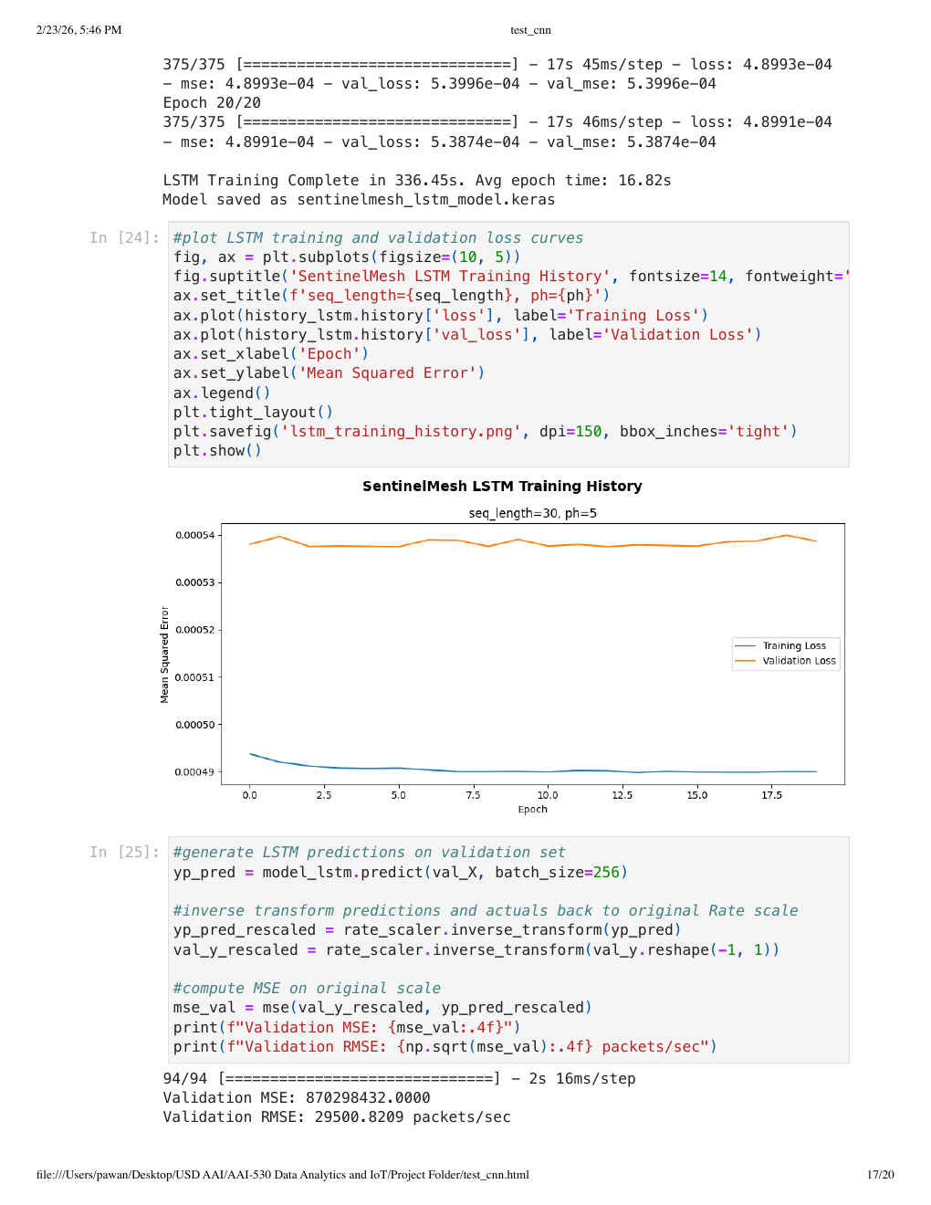
The model struggled to track sharp traffic-rate spikes. The prediction line stayed relatively flat while actual traffic had sudden bursts.
At first, that seems like a failure. But from a security perspective, it still has value.
If the model learns a normal baseline and live traffic suddenly moves far above that baseline, the prediction error becomes an anomaly signal.
The biggest lesson: outliers matter
The Rate feature had extreme outliers. When using MinMaxScaler, those outliers compressed most normal values near zero.
That caused the LSTM to learn a near-flat baseline.
In a future version, I would improve this with:
- 99th-percentile clipping before scaling
- RobustScaler instead of MinMaxScaler
- Per-device baselines
- Rolling-window thresholds
- Dynamic thresholds instead of static thresholds
- Separate models for different IoT device types
This is an important lesson: the model architecture is only one part of the system. The preprocessing pipeline can make or break the result.
Step 7: Turn predictions into anomaly alerts
Once the LSTM predicts a rate value, we can compare the prediction to the actual observed rate.
prediction_error = abs(actual_rate - predicted_rate)
Then we can define a threshold.
if prediction_error > threshold:
    anomaly = True
else:
    anomaly = False
A more production-ready version would calculate thresholds dynamically.
Example:
threshold = rolling_mean_error + (2 * rolling_std_error)
This allows the threshold to adapt as normal traffic changes.
Step 8: Fuse CNN and LSTM signals
The real power of SentinelMesh comes from combining both models.
The CNN gives a threat probability.
The LSTM gives an anomaly signal.
A simple decision-fusion engine can combine both.
def classify_alert(cnn_score, lstm_error, threshold):
    if cnn_score >= 0.90 and lstm_error > threshold:
        return "critical"
    elif cnn_score >= 0.75:
        return "high"
    elif lstm_error > threshold:
        return "warning"
    else:
        return "normal"
This gives four useful states:
normal   = no strong model signal
warning  = abnormal rate pattern
high     = suspicious flow classification
critical = suspicious flow + abnormal rate spike
This is closer to how real security systems work. They rarely depend on one signal alone. They combine multiple indicators and assign severity.
Step 9: Build the dashboard
A security system is not useful if analysts cannot understand the output.
So I created a dashboard with four main views:
- Total threats detected
- Threat summary by attack label
- CNN confusion matrix
- LSTM actual vs predicted rate forecast
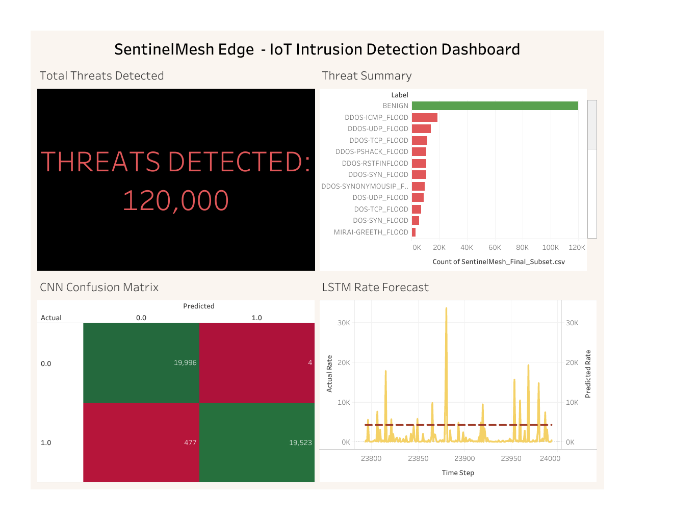
The dashboard turns the model output into something closer to SOC workflow.
Instead of only showing model accuracy in a notebook, it shows:
- How many threats were detected
- Which attack types appeared most often
- Where the CNN made mistakes
- Whether the LSTM baseline is seeing abnormal spikes
What I would improve next
If I were turning SentinelMesh into a production-grade system, my next improvements would be:
Multi-class attack detection
The current CNN is binary: benign or attack. A stronger version would classify specific attack types such as DDoS, spoofing, scanning, brute force, and web-based attacks.
Per-device behavior modeling
A smart camera and a smart thermostat should not share the exact same baseline. Each device type should have its own normal behavior profile.
Better LSTM preprocessing
The LSTM should use outlier clipping, robust scaling, and possibly multiple features instead of only traffic rate.
SIEM integration
Alerts should flow into a SIEM such as Splunk, Microsoft Sentinel, or Elastic.
Example alert:
{
  "device_id": "camera-001",
  "cnn_score": 0.97,
  "lstm_error": 18422.5,
  "severity": "critical",
  "action": "isolate_device"
}
Automated response
A future version could trigger actions such as:
- Block source IP
- Isolate IoT device VLAN port
- Disconnect MQTT session
- Create SIEM incident
- Notify SOC analyst
Final thoughts
SentinelMesh started as an AI/IoT project, but the bigger lesson was about building security systems.
A good AI security system is not just a model. It needs architecture, data pipelines, preprocessing, inference, alerting, dashboards, and operational feedback.
The CNN gave SentinelMesh a strong attack classifier. The LSTM added anomaly-detection behavior. The dashboard made the results understandable.
Together, those pieces create the foundation for an edge AI intrusion detection system for IoT networks.